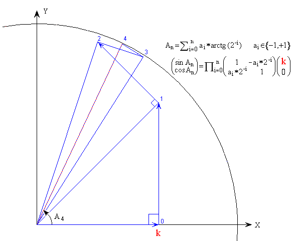
Sine and Cosine computation
|
Sine and Cosine |
|
From weighting a bread loaf to sine and cosine computation |
We want to compute sine( A ) and/or cosine ( A ); we have available a scale, a white bread whose weight is actually just A and a set of weights with values arctg ( 2-j ). All the weights must go on the scale plates, either side. |
|
Sine and Cosine computation |
Let Vj be a vector, with extremity (Xj, Yj). A "pseudoRotation" of an
angle arctg (2-j ) applied to Vj gives Vj+1 : Xj+1 = Xj Yj
* 2-j and Yj+1 = Yj + Xj * 2-j. A "pseudoRotation"
of an angle -arctg (2-j ) applied to Vj gives Vj+1 : Xj+1 = Xj + Yj
* 2-j and Yj+1 = Yj Xj * 2-j. After
the angle A is broken down into a weighted sum of arctg (2-j ), a series of "pseudoRotations"
yields the coordinates of the vector of angle A, those coordinate are the values sin(A) and cos(A) searched for.
All the "pseudoRotations" require only addition/subtraction and shift. |
|
Angle decomposition |
What is the domain of the angles A = S i ai arctg (2-i) and what precision can be expected from this notation ? A is the angle value to reach, and T is the value attained by the series of "pseudoRotations". To change the value of A, click in the figure. All values are expressed in radiant. The key "Reset" allow to control manually the convergence into the notation arctg (2-i) by clicking the digit values. |
|
The constant k |
Each "pseudoRotation" of the angle arctg(2-j ) brings about a vector lengthening of
Ö1+2-2j, for it is not exactly a rotation but rather a displacement
of the vector extremity on a perpendicular vector. In order to compensate in advance the product of all the lengthening
of a series of "pseudoRotations", the starting vector is ( X0 = k
, Y0 = 0 ) . For n large enough, k is approximately equal to 0,60725. In order
for k to be a constant, the representation with arctg(2-j ) use digits
Î{ '-1' , '1' }.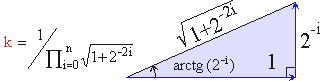 |
|
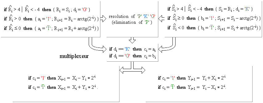
"Robertson's diagram" for CORDIC |
The "Robertson's diagram" shows that the iteration to convert into
basis arctg(2-j ) may be as follows: |
|
"non restoring" divider for CORDIC |
The angle V (divider's top) is in the interval [ -1.0.. +1.0 [ . The constant bits at "AS" cells inputs are wired. The operations are selected according to the previous partial remainder R or by V0 for the first iteration . |
| If the "PseudoRotations" use carry-propagation-free additions/subtractions
(here the "CS") then the delay is given by the stage number. The first stage does not have to perform
an addition/subtraction since X0 = k , Y0 = 0, and consequently if a0 = '1' then { X1 = k ; Y1 = k } else { X1 = k ; Y1 = - k }. and for all the subsequent steps if aj = '1' then {Xj+1= Xj Yj* 2-j ; Yj+1= Yj + Xj* 2-j } else {Xj+1= Xj + Yj* 2-j ; Yj+1= Yj Xj* 2-j }. To keep the picture clear, the wires Xj * 2-j are not always drawn. |
|
"RO" cell |
The "RO" cell is a variant of the addition cell "CS" with an extra input "aj" to control either the addition or the subtraction. Notice that the activity of the input carry "e" never propagates to the output carry "h".
|
|
"Robertson's diagram" for "double rotation" CORDIC |
All the constants arctg(2-j) fall inside the interval [ 0,7853982.. 1 [ . Thus there are normalized
and a carry-propagation free divider can be used. It uses an approximation
|
|
"double rotation" CORDIC |
This divider uses the same "head" and "tail" cells as the "SRT" divider. To put up with the '0', the angle is first halved then the "pseudoRotation" are doubled. Thanks to that, the lengthening stays the same (Ö1+ 4-i )2 for each of the three possible values of aj .
|
|
Reduced constants |
All the constants arctg(2-j) are in the interval [ 0.7853982.. 1 [ . Their binary representation always starts with 0.11. If the constants are all multiplied by 0.75 they all fall in the interval [ 0.58904865.. 0,75 [ and their binary representation now starts with 0.10. The decomposition of angle V does not changes if it is also multiplied by 0.75 thanks to the positive and negative divider inputs. The "head" in now simpler and thus the circuit is faster. |
| The constant k for the double double rotation is the square of the preceding k. Moreover the double rotation computes sin(2*A) and cos(2*A). Angle A must be divided by 2 (a shift) prior to the "SRT" division. |
|
Operator for the double "PseudoRotation" |
For each digit aj , two "PseudoRotations" of angle arctg(2-j) are performed carry propagation free. |
| The "double rotation" has a cost: it doubles the rotation hardware and probably the delay as well. Is it possible to obtain a quotient written with digits aj Î{ '1', '-1' } with a delay similar to the division for the double rotation ? The quotient converter works with weights 2-j since then '0' '1' = '1' '-1' but this is no longer true weights arctg(2-j ) . |
The "double division" is more ingenious. It makes use of two dividers running simultaneously with slightly
different "head" cells.
Only divider1 is shown by the following applet yet both are simulated. |
| The two heads detect the overflow to produce together a 3-valued indicator : 'K' the output digit aj is correct (divider2 overflows), 'G' the output digit bj is correct (divider1 overflows), 'P' propagate the next indicator's value (no overflow, aj and bj are both acceptable so far). Whenever a divider overflows, it carries on with the other divider's partial remainder R. The propagation is similar to the carry propagation of addition. The on-the-fly quotient converter is well suited. |
|
Tangent computation |
To compute the tangent, the sine and cosine are first computed, then their quotient. Nevertheless the constant k has no incidence on the quotient. The rotation starts with X0 = 1 , Y0 = 0, and the "pseudoRotations" operator is simplified accordingly . |